Building up an ERP
Event-related potentials are one of the simplest ways of representing event-locked EEG data. Imagine a very simple visual experiment in which participants have to respond to pictures of objects. You set up the experiment so that an event trigger is sent to your EEG recording system at the time the picture flashes up screen. Then, afterwards, you extract epochs around those triggers to get a bunch of seperate epochs, each time-locked to the onset of the stimulus. You then average across those epochs in the time-domain, et voila! You have an ERP.
Here’s a couple of quick examples from a dataset that’s included in my package, eegUtils.
erp_demo <- rm_baseline(demo_epochs, c(-.1, 0))
plot_butterfly(erp_demo) +
  plot_timecourse(erp_demo, "A29") +
  ggtitle("A29") +
  topoplot(erp_demo, c(.1,.11), chan_marker = "name") +
  plot_layout(ncol = 2)
## Using electrode locations from data.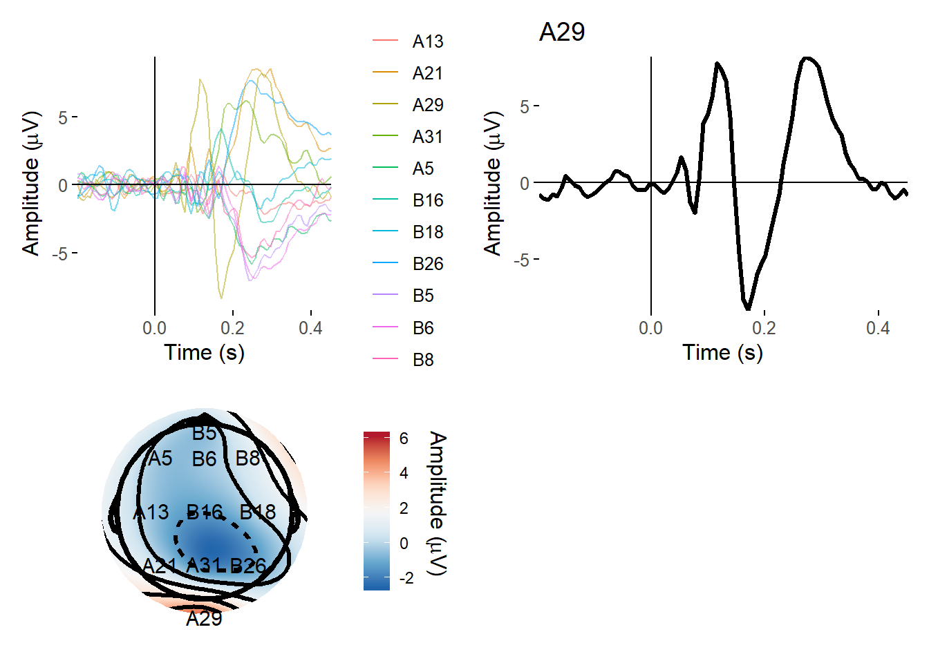
On the left we have a butterfly plot showing the ERP at each of the 11 electrodes included in this dataset. Note that this was an experiment in which participants saw pictures of objects and non-objects, but the details are not important here. We have a clear and very typical ERP here; I isolate one electrode - A29, which is over occipital cortex, and you can clearly see a P1 and N1 complex going on.
How does this look at the single trial level? One way to look it is to overlay all the single epochs on each other!
Trial-by-trial overlay
Here I use the package gganimate to layer each consecutive trial on top of the other.
erp_demo <- as.data.frame(erp_demo)
epo_by_epo <- ggplot(erp_demo,
                     aes(x = time,
                         y = A29)) +
  geom_line() +
  transition_time(epoch) +
  shadow_mark(colour = "grey",
              alpha = 0.7) +
  theme_classic(12) +
  labs(title = "epoch: {frame_time}",
       x = "Time (s)")

animate(epo_by_epo,
        nframes = 80,
        fps = 5)
As you’ll be able to see, there’s substantial variability from trial to trial, but over time you can see more and more of the familiar structure emerge in the background.
Trial-by-trial averaging
How does that build up into the ERP over time? How long does it take for that structure to stabilize? You might expect that more and more is better and better. But the contribution of each trial to the ERP tails off
For the next plot, I plot instead the cumulative average ERP. So first I plot one epoch, then take the average of that and the next epoch, and so and so on.
erp_demo <- erp_demo %>%
  group_by(time) %>%
  mutate(avg_erp = cummean(A29))

cumul_epos <- ggplot(erp_demo,
                     aes(x = time,
                         y = avg_erp)) +
  geom_line() +
  transition_time(epoch) +
  shadow_mark(colour = "grey",
              alpha = 0.7) +
  theme_classic(12) +
  labs(title = "epoch: {frame_time}",
       x = "Time (s)")
animate(cumul_epos,
        nframes = 80,
        fps = 5)
After around 20 epochs or so, the ERP really starts to settle down, and doesn’t change an awful lot thereafter. It’s noticeable that the average starts off higher and then gradually reduces. Of course, this can’t be taken as being what happens in every case - it depends on the amplitude and variability of the components you’re studying.
But what it does show is how the improvements in signal-to-noise ratio are not everlasting with increasing numbers of epochs. The more epochs you have, the less each individual epoch contributes to the average, and the more epochs you’d need to noticeably shift the ERP.
In fact, there’s a simple equation, if S is the signal, R is the noise, and N is the number of trials, then the size of the noise in each individual trial is a equal to (1 / sqrt(N)) * R. Thus, noise decreases as a function of the square root of the number of trials, and conversely, the SNR increases. [^1]
[^1] See Luck, S.J. Ten Simple Rules for Designing and Interpreting ERP experiments
Matt Craddock
I'm a research software engineer