Importing BDF files in R - referencing and filtering
At my recent workshop, several people asked about pre-processing of data in R, and I told them it wasn’t really possible at the moment. What I might have been less clear about is that it is not that is not possible, but that there isn’t really the wide range of pre-programmed tools as in Python and Matlab. So it’s just not practical to do it all in R as it stands.
But I’ve never been one to let practicality bother me that much.
One thing that I had tried in the past but found to be very slow was a package for reading EDF/BDF files - edfReader. BDF is the recording format of the BioSemi ActiveTwo system, one of the most popular research grade recording systems, and the one I’m currently using. Having been asked about this, I thought I’d try it out again. It’s not quite as slow as I remember.
The first step is to load in the header of the file. The header contains lots of useful information - the number of signals, the filepath, the channel labels, filter settings
## File name            : C:\Users\Matt\Dropbox\BlogStuff\EEG_data\S123ExteroSSDTB1.bdf
## File type            : BDF
## Version              : "255"BIOSEMI
## Patient              :
## RecordingId          :
## StartTime            : 2017-02-03 14:46:18
## Continuous recording : TRUE
## Recorded period      : 374 sec = 00:06:14 hⓜs
## Ordinary signals     : 73
## Annotation signals   : 0
## Labels               : Fp1, AF7, AF3, F1, F3, F5, F7, FT7, FC5, FC3, FC1, C1, C3, C5, T7, TP7, CP5, CP3, CP1, P1, P3, P5, P7, P9, PO7, PO3, O1, Iz, Oz, POz, Pz, CPz, Fpz, Fp2, AF8, AF4, AFz, Fz, F2, F4, F6, F8, FT8, FC6, FC4, FC2, FCz, Cz, C2, C4, C6, T8, TP8, CP6, CP4, CP2, P2, P4, P6, P8, P10, PO8, PO4, O2, EXG1, EXG2, EXG3, EXG4, EXG5, EXG6, EXG7, EXG8, Status
bdf_header <- readEdfHeader("F:\\Dropbox\\BlogStuff\\EEG_data\\S123ExteroSSDTB1.bdf")
summary(bdf_header)The data itself is loaded in using readEdfSignals(). I tell it to load only “Ordinary” signals - there is another signal type called “Annotations”, but they don’t seem to be anything meaningful.
start <- proc.time()
test_data <- readEdfSignals(bdf_header, signals = "Ordinary")
end <- proc.time()-start
end
## user system elapsed
## 28.81 2.04 31.69This took ~31.69 seconds, which is not too bad, but for comparison loading the same file in Matlab using the Biosig toolbox takes ~5 seconds. My previous attempt at using this package took several minutes to load a similar file, so either I was doing something wrong or the package has been updated since then. At some point I might investigate the function and see if I can speed it up, but it’s not slow enough for me to care too much right now.
What you end up with is a nested list structure, with an entry for each electrode - in this case, 64 scalp electrodes with 8 externals (actually only 6 in use) - and the Status channel, which is where all the triggers are stored.
The complexity and redundacy of this list structure might be part of why this is slower than the Matlab command, which returns a much more pared down structure. Each entry for each electrode contains all the same info regarding, for example, prefiltering, bitrate, and sample rate. This is highly redundant as it is the same for every electrode.
Here’s an example of the list entry for one electrode.
test_data[[1]]## R signal : 1
## Name : Fp1
## Start time : 2017-02-03 14:46:18
## Continuous recording : TRUE
## Recorded period : 374 sec = 00:06:14 hⓜs
## Period read : whole recording
## Sample rate : 1024 /sec
## Number of samples : 382976The actual recordings are stored in a list called signal nested within the list for each electrode.
Happily, we can trivially turn this list into a dataframe with one column for each electrode (and the status channel) using map_df() from purrr and one row per sampling point.
data_df <- map_df(test_data,"signal")
head(data_df)
## # A tibble: 6 x 73
## Fp1 AF7 AF3 F1 F3 F5 F7 FT7 FC5 FC3 FC1
## <dbl> <dbl> <dbl> <dbl> <dbl> <dbl> <dbl> <dbl> <dbl> <dbl> <dbl>
## 1 13214. -5049. -6476. -404. -3308. -4940. -9600. -10487. -5016. 3164. 1499.
## 2 13215. -5048. -6475. -405. -3308. -4940. -9599. -10488. -5017. 3165. 1499.
## 3 13210. -5051. -6479. -408. -3311. -4944. -9601. -10488. -5019. 3162. 1496.
## 4 13209. -5052. -6478. -405. -3309. -4942. -9600. -10486. -5015. 3166. 1499.
## 5 13207. -5051. -6475. -403. -3306. -4938. -9599. -10484. -5011. 3170. 1503.
## 6 13210. -5045. -6470. -399. -3301. -4930. -9593. -10476. -5006. 3175. 1508.
## # ... with 62 more variables: C1 <dbl>, C3 <dbl>, C5 <dbl>, T7 <dbl>,
## # TP7 <dbl>, CP5 <dbl>, CP3 <dbl>, CP1 <dbl>, P1 <dbl>, P3 <dbl>, P5 <dbl>,
## # P7 <dbl>, P9 <dbl>, PO7 <dbl>, PO3 <dbl>, O1 <dbl>, Iz <dbl>, Oz <dbl>,
## # POz <dbl>, Pz <dbl>, CPz <dbl>, Fpz <dbl>, Fp2 <dbl>, AF8 <dbl>, AF4 <dbl>,
## # AFz <dbl>, Fz <dbl>, F2 <dbl>, F4 <dbl>, F6 <dbl>, F8 <dbl>, FT8 <dbl>,
## # FC6 <dbl>, FC4 <dbl>, FC2 <dbl>, FCz <dbl>, Cz <dbl>, C2 <dbl>, C4 <dbl>,
## # C6 <dbl>, T8 <dbl>, TP8 <dbl>, CP6 <dbl>, CP4 <dbl>, CP2 <dbl>, P2 <dbl>,
## # P4 <dbl>, P6 <dbl>, P8 <dbl>, P10 <dbl>, PO8 <dbl>, PO4 <dbl>, O2 <dbl>,
## # EXG1 <dbl>, EXG2 <dbl>, EXG3 <dbl>, EXG4 <dbl>, EXG5 <dbl>, EXG6 <dbl>,
## # EXG7 <dbl>, EXG8 <dbl>, Status <dbl>A couple of things to consider about this data are that BioSemi data is recorded with a low-pass filter only (in this case, at 208 Hz), and is referenced to two channels which are not present in the data - Common Mode Sense (CMS) and Driven Right Leg (DRL). All the channels thus end up with different DC offsets and with noise spread across them from the reference channel. We need to re-reference the data and to high-pass filter it.
Re-referencing data
Let’s re-reference to the average reference. For that we need to subtract the mean of all channels at each sampling point from each channel at each sampling point. This being R, there are a bunch of different ways we could do this. The simplest way is to use rowMeans() and subtract the resulting vector from each column. In our data frame, only the first 70 columns actually have real data on them.
Here’s a comparison of the data from electrode Fp1 before and after average referencing.
avg_ref <- data_df
avg_ref[,1:70] <- avg_ref[,1:70] - rowMeans(avg_ref[,1:70])

data_df %>%
  rowid_to_column("sample") %>%
  filter(sample <= 400) %>%
  select(sample, Fp1) %>%
  ggplot(aes(x = sample, y = Fp1)) + geom_line() + ggtitle("Before")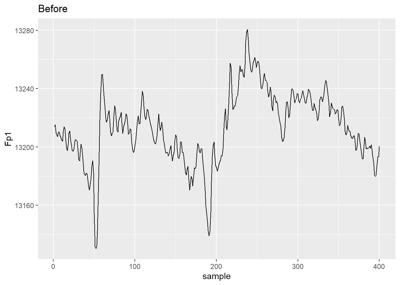
avg_ref %>%
  rowid_to_column("sample") %>%
  filter(sample <= 400) %>%
  select(sample, Fp1) %>%
  ggplot(aes(x = sample, y = Fp1))+ geom_line() + ggtitle("After")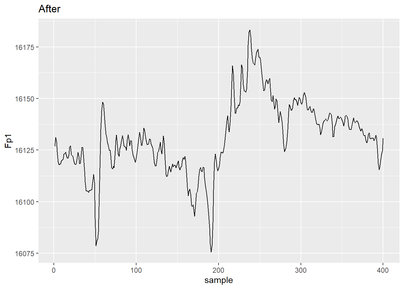
Note you could easily apply any referencing scheme you wanted - e.g. averaged mastoids.
Filtering
We still need to do some filtering. Helpfully there is a package called signal that implements Matlab/Octave style filters. In recent years this implementation has been replaced in EEGLAB and Fieldtrip by Andreas Widmann’s filtering plugin, but to we’ll try the older, legacy versions out, as I’d need to recreate the newer code here. I dug around in the EEGLAB code to find out the default settings of its legacy filtering code.
We’ll do a high-pass FIR filter with a passband edge at 1 Hz. By default, we use a Hamming window of order 3 * (sampling rate/ frequency of the lower edge of the passband). From that, fir1() creates a set of filter weights for use by filtfilt(). filtfilt() filters the signal twice - once forwards, once in reverse - so that it performs zero-phase filtering and does not shift the signal in time.
First we create a set of filter coefficients using fir1().
library(signal)
low_edge <- 1
sRate <- test_data$Fp1$sRate
filt_ord <- 3 * (sRate/low_edge)
filt_coef <- fir1(filt_ord, low_edge/(sRate/2), type = "high")
The R filtfilt() implementation only operates on vectors, not on dataframe columns, so we’ll take a column from our average referenced dataframe and apply it to that column.
Fp1_vec <- as.numeric(unlist(avg_ref[[1]]))
Fp1_filt <- filtfilt(filt_coef, Fp1_vec)
plot(Fp1_filt, type = "l")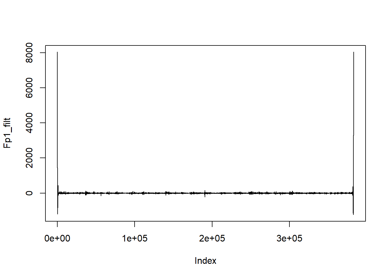
There’s an obvious problem here - massive edge effects. The filtering process assumes that the signal is zero outside the edges of the actual signal, which creates huge offsets when the ends of the signal are not actually zero. The Matlab version of filtfilt mitigates edge effects by mirroring the signal at each end so that no massive offsets are created - it takes the first and last n (actually, filter length*3) samples, reverses them, then adds them to the end of the signal. After filtering, these sections are removed, leaving only samples from the original timerange. This doesn’t happen in the R version of the command, so we get huge edge effects.
Fp1_mirror <- c(rev(head(Fp1_vec, 3 * length(filt_coef))),
                as.numeric(unlist(avg_ref[[1]])),
                rev(tail(Fp1_vec, 3 * length(filt_coef))))
Fp1_mirror_filt <- filtfilt(filt_coef, Fp1_mirror)
Fp1_filtered <- Fp1_mirror_filt[(3 * length(filt_coef) + 1):(3 * length(filt_coef)+1000)]
plot(Fp1_filtered, type = "l")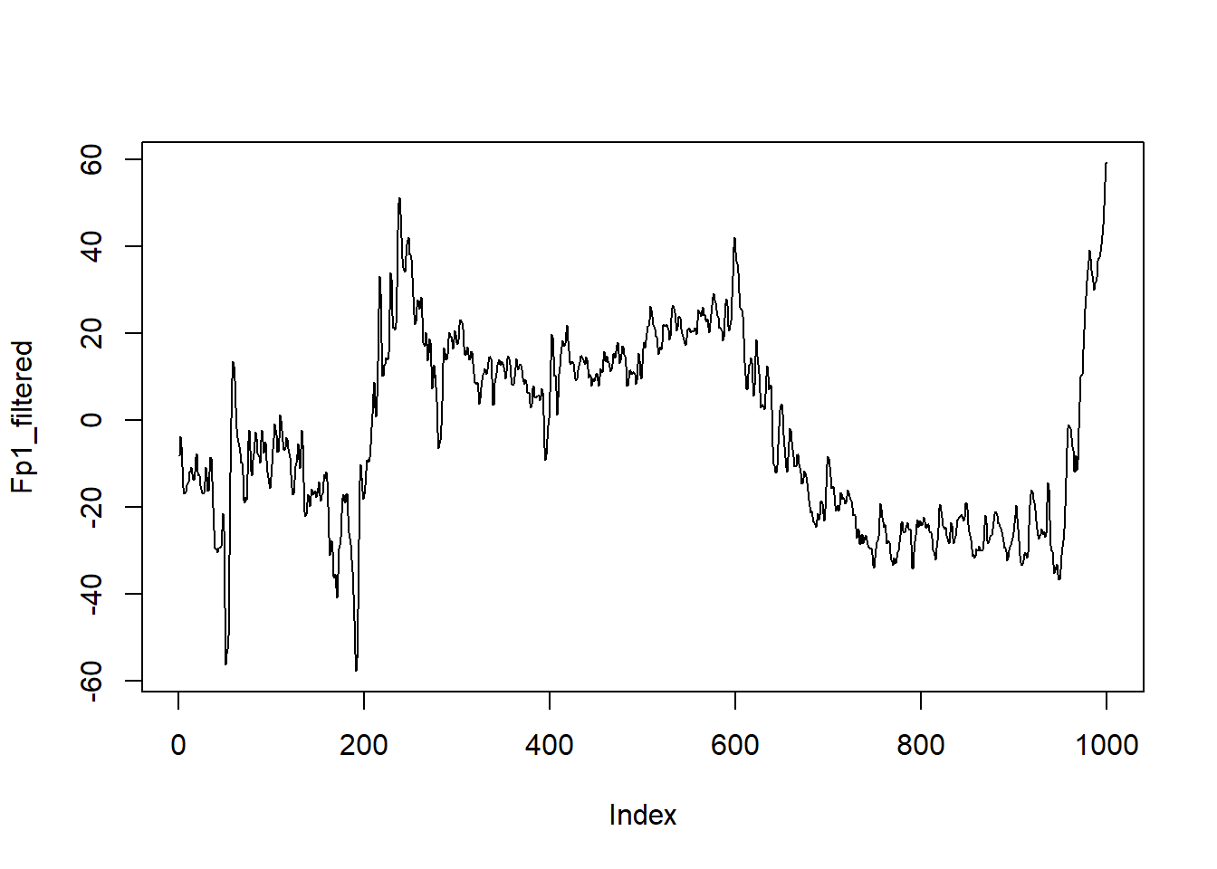
Of course, we don’t want to do this to just one channel, but to all of them. Since this gets a little fiddly, what with the unlisting and mirroring etc, let’s write a custom function to do it.
filt_func <- function(x, filt_coef) {
  tmp_dat <- as.numeric(unlist(x))
  mirror_dat <-  c(rev(head(tmp_dat, 3 * length(filt_coef))),
                tmp_dat,
                rev(tail(tmp_dat, 3 * length(filt_coef))))
  filt_dat <- filtfilt(filt_coef, mirror_dat)
  trim_dat <- filt_dat[(3 * length(filt_coef)  +1):(length(filt_dat) - (3 * length(filt_coef)))]
}
This function unlists the data column and turns it into a vector, pads it with mirrored signals at each end, filters it, then cuts off the padding. It returns a filtered vector.
We then run that on each electrode separately.
start <- proc.time()
filt_dat <- avg_ref %>%
  rowid_to_column("Samp_No") %>%
  gather(electrode, amplitude, -Samp_No, -Status) %>%
  nest(-electrode) %>%
  mutate(filt_amp = map(data,
                        ~filt_func(.$amplitude, filt_coef))) %>%
  unnest()
## Warning: All elements of `...` must be named.
## Did you want `data = c(Samp_No, Status, amplitude)`?## Warning: `cols` is now required.
## Please use `cols = c(data, filt_amp)`end <- proc.time()-start
end## user system elapsed
## 639.21 11.55 655.86So that took ~10.931 minutes. That’s really slow - the same process took around 3 minutes in Matlab. Widmanns’ EEGLAB method is much faster anyway, so perhaps implementing that would speed things up. And it’s an embarrassingly parallel task that should speed up significantly if split across multiple CPU cores, but I’ll leave that for another post.
Let’s plot the fruits of our labours - the unfiltered and filtered data.
Note that here we run into a conflict of function names. Because I loaded signal after I loaded tidyverse, R uses the filter() command from signal. By adding dplyr:: before filter(), I make sure it uses the right one.
filt_dat %>%
  dplyr::filter(Samp_No <= 15000 & !(electrode == "EXG7"| electrode == "EXG8")) %>%
  gather(filtered, amplitude, filt_amp, amplitude) %>%
  ggplot(aes(x = Samp_No, y = amplitude, group = interaction(electrode,filtered), colour = filtered)) + geom_line(alpha = 0.5)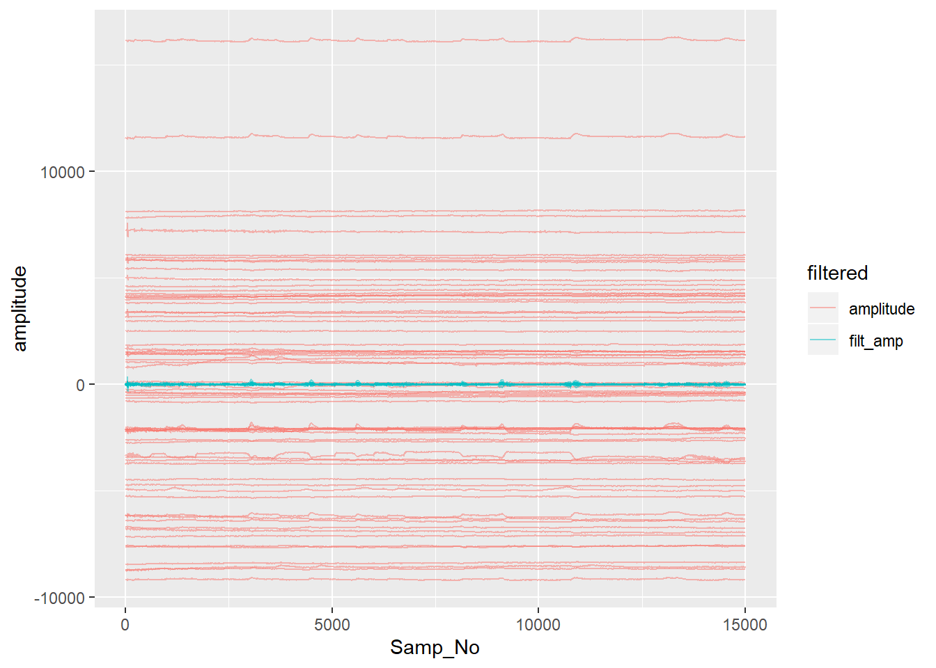
Note how the filtered data is clustered around zero - filtering removed the DC offset in the raw data.
If we remove the DC constant from each channel in the raw data by simply subtracting each channel’s mean, we can see a little better the other differences made by filtering.
filt_dat %>%
  dplyr::filter(Samp_No <= 15000 & !(electrode == "EXG7"| electrode == "EXG8")) %>%
  group_by(electrode) %>%
  mutate(amplitude = amplitude - mean(amplitude)) %>%
  ungroup() %>%
  gather(filtered, amplitude, filt_amp, amplitude) %>%
  ggplot(aes(x = Samp_No, y = amplitude, group = interaction(electrode,filtered), colour = filtered)) + geom_line(alpha = 0.5)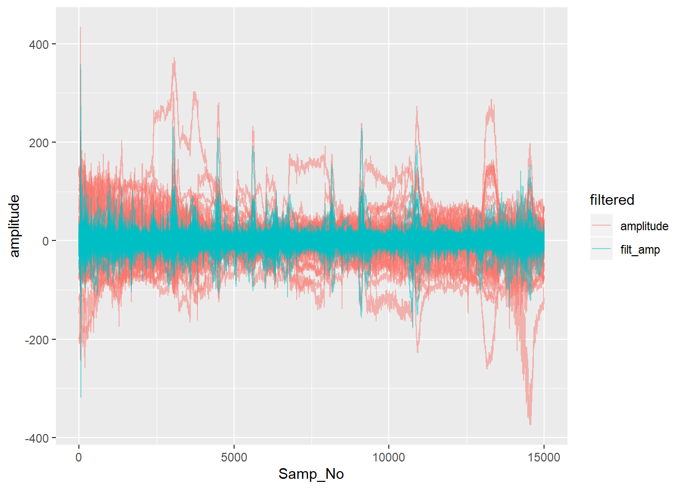
Of course, this isn’t the end of pre-processing. We haven’t dealt with epoching or artefact rejection. My next post will take a look at processing the Status channel and turning it in a record of which trigger occurred when, and epoching the data.
Matt Craddock
I'm a research software engineer