Importing BDF files in R - Events and epoching

Trigger events

A Biosemi system can record up to 16 trigger inputs, representing the resulting numbers as 16-bit (i.e from 0-65535 coded in binary format). The status channel actually uses 24-bits, with the bits above 16 used for things like signalling that the battery is low or that the signal from CMS is in or out of range. The triggers I used were all in the range 0-256, since they were sent using the parallel port - the parallel port only uses 8-bits for sending data. Thus the format of the triggers in the recording does not necessarily correspond to the format of the triggers you sent. All we need to do is a modulo operation (%% in R) to get the remainder after dividing by 65536, and we have our original trigger numbers back.

unique(data_df$Status)

##  [1] -6750208 -6749955 -6815744 -6815728 -6815644 -6815743 -6815730 -6815732
##  [9] -6815616 -6815740 -6815742 -6815734 -6815741

unique(data_df$Status) %% (256*256)

##  [1]   0 253   0  16 100   1  14  12 128   4   2  10   3

Let’s replace the status column with sensible triggers. In reality it’s probably also best to have the Status channel split off, rather than duplicating it for every channel in a long format representation, or to just treat it as another channel. I won’t bother with either of those things here though. Let’s also plot part of our Status channel to get a feel for the structure of the events.

avg_ref$Status <- avg_ref$Status %% (256*256)

avg_ref %>%
  rowid_to_column("Samp_No") %>%
  dplyr::filter(Samp_No >= 2000 & Samp_No <= 50000) %>%
  ggplot(aes(x = Samp_No, y= Status, colour = Status))+
  geom_point()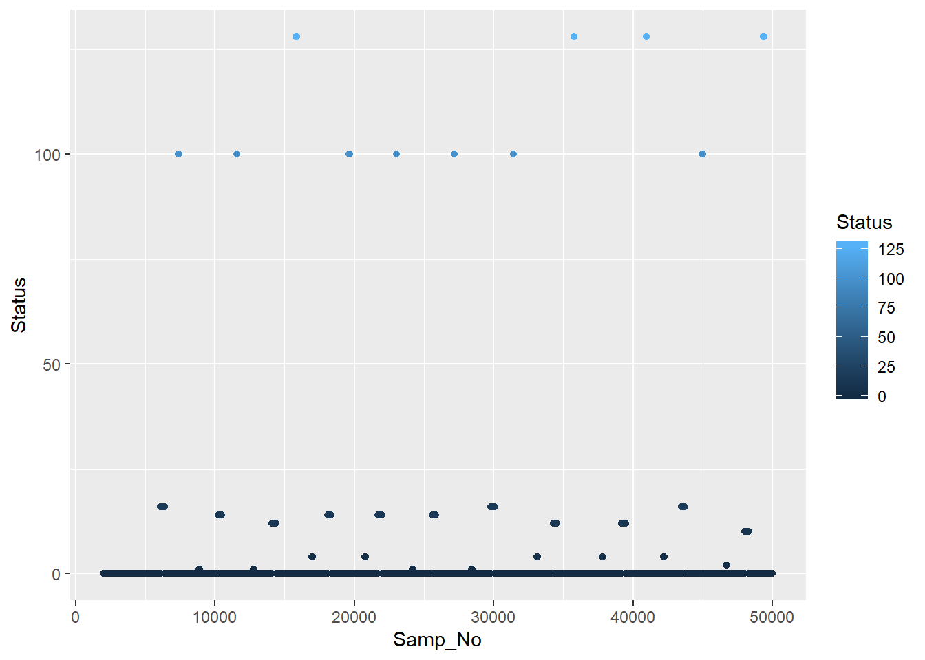

A couple of things you might notice are all the zeros along the bottom and that the triggers are usually a run of points, rather than one single point. When you send a trigger, you are essentially flipping a switch that stays up until it’s switched down again. Really we want to only keep the first trigger in a chain.

If we take the difference of each consecutive value in the status channel, we end up with a vector which is set to zero when there is no change, a positive number when there is an increase (trigger onset), and a negative number when there is a decrease (trigger offset). Using the which() command, I find the index of the trigger onsets in the difference vector, and add 1 to it to account for the differencing operation.

events_diff <- diff(avg_ref$Status)
event_table <- data.frame(event_onset = which(events_diff > 0)+1,
                          event_type = avg_ref$Status[which(events_diff > 0)+1])
head(event_table,10)

##    event_onset event_type
## 1          966        253
## 2         6111         16
## 3         7399        100
## 4         8851          1
## 5        10234         14
## 6        11569        100
## 7        12774          1
## 8        14115         12
## 9        15826        128
## 10       16977          4

I now have a table giving the onset time (in samples) of each trigger in the data, and the type of each trigger. I have validated these against the same file imported in EEGLAB.

Now I’ll plot some data with vertical lines added when each trigger occurs, with the lines coloured and labelled according to which trigger type they were.

filt_dat %>%
  dplyr::filter(Samp_No <= 15000 & !(electrode == "EXG7"| electrode == "EXG8")) %>%
  ggplot(aes(x = Samp_No, y = filt_amp, colour = electrode)) +
  geom_line(alpha = 0.5) +
  geom_vline(xintercept = event_table[event_table$event_onset <= 15000, ]$event_onset,
             linetype = "dashed",
             colour = event_table[event_table$event_onset <= 15000, ]$event_type) +
  scale_x_continuous(sec.axis = sec_axis(trans = ~.,
                                         breaks = event_table[event_table$event_onset <= 15000,]$event_onset,
                                         labels = event_table[event_table$event_onset <= 15000,]$event_type))

## Warning: Detecting old grouped_df format, replacing `vars` attribute by `groups`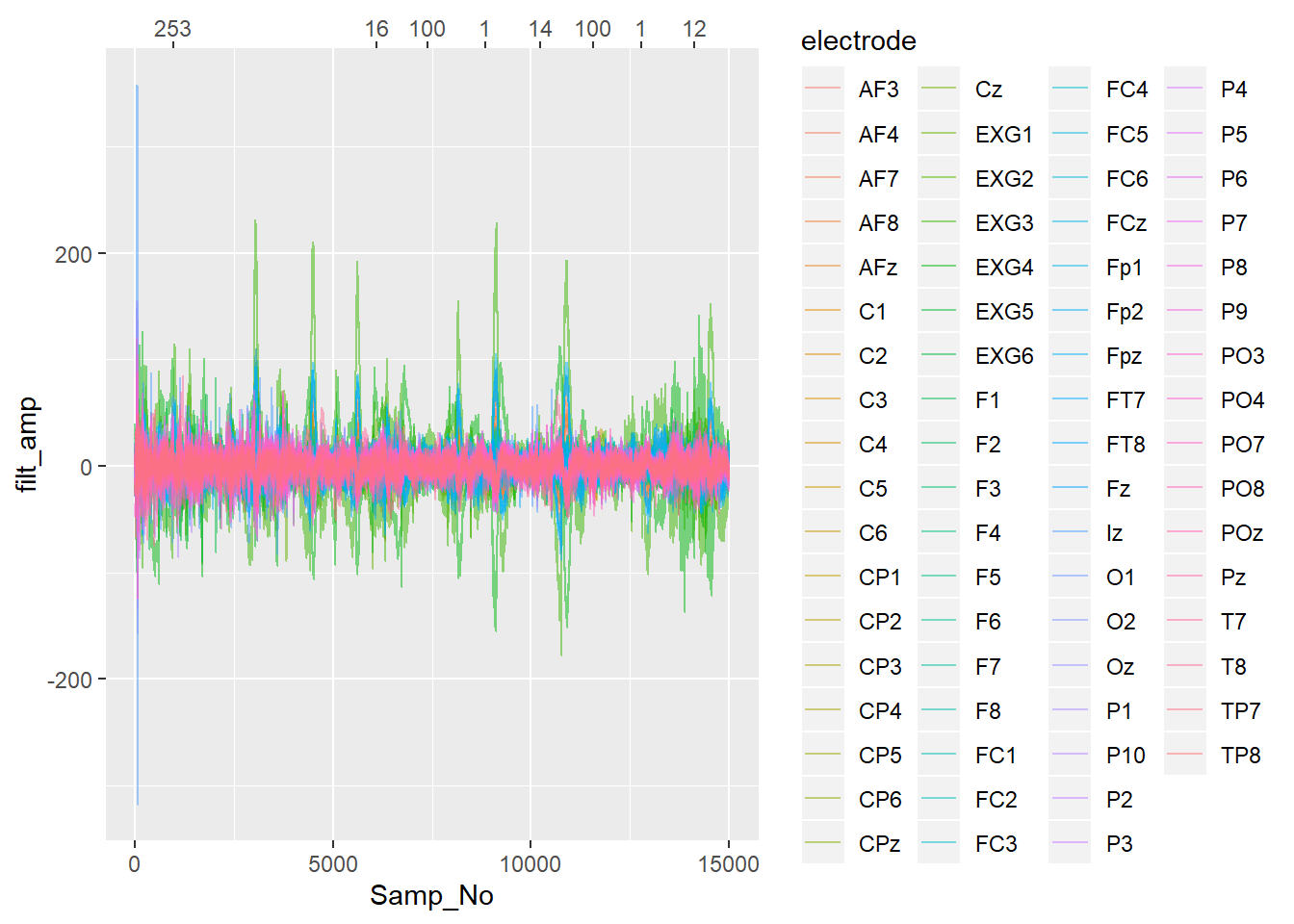

Epoching

Suppose now we want to form epochs around one of the triggers; around, say, trigger 100. These epochs should start 200 ms before the trigger until 500 ms after it.

First we create a vector of samples the cover the time range around our time-locking event.

lower_lim <- -.2
upper_lim <- .5
samps <- seq(round(lower_lim * 1024), round(upper_lim * (1024-1)))
samps[1:10]

##  [1] -205 -204 -203 -202 -201 -200 -199 -198 -197 -196

Then we can create our epochs by choosing the time-locking events from the event table we made earlier. Those will be the zero point in our epochs, and are coded as the sample number in the original dataset. We then take our sample vector created in the last code chunk and add that vector to our vector of time-locking events. Here I use map to step through each item in the vector and output a list containing the sample numbers for each epoch. I then pass that list down and create a dataframe of the sample numbers for each epoch, the times those points convert into relative to our timelocking event, and an epoch number for each epoch. Finally, I join that up with our filtered, average referenced continuous data, picking out only those timepoints that belong to one of our epochs.

## # A tibble: 27,574,272 x 4
##    electrode filt_amp Samp_No Status
##    <chr>        <dbl>   <int>  <dbl>
##  1 F5            5.33       1      0
##  2 F5            8.21       2      0
##  3 F5            7.38       3      0
##  4 F5            5.91       4      0
##  5 F5            6.61       5      0
##  6 F5            9.98       6      0
##  7 F5            9.80       7      0
##  8 F5            8.18       8      0
##  9 F5            8.14       9      0
## 10 F5            8.47      10      0
## # ... with 27,574,262 more rows

epoch_zero <- event_table[which(event_table$event_type == 100),]$event_onset

epoched_data <- map(epoch_zero, ~(. + samps)) %>%
  map_df(~data.frame(Samp_No = ., Time = samps/1024), .id = "epoch_no") %>%
  left_join(filt_dat)

## Joining, by = "Samp_No"

head(epoched_data)

##   epoch_no Samp_No       Time electrode   filt_amp Status
## 1        1    7194 -0.2001953        F5 -1.1852892      0
## 2        1    7194 -0.2001953       FT7  1.0523597      0
## 3        1    7194 -0.2001953       FC1 -1.5428764      0
## 4        1    7194 -0.2001953       TP7  0.4129892      0
## 5        1    7194 -0.2001953       CP5 -1.6642918      0
## 6        1    7194 -0.2001953       CP1  3.0524871      0

We now have an epoched dataset, time-locked to our trigger of interest.

ERPs <- epoched_data %>%
  filter(!grepl("^E",electrode)) %>%
  group_by(electrode,Time) %>%
  summarise(amplitude = mean(filt_amp)) 

ggplot(ERPs, aes(x = Time, y = amplitude, colour = electrode)) +
  geom_line()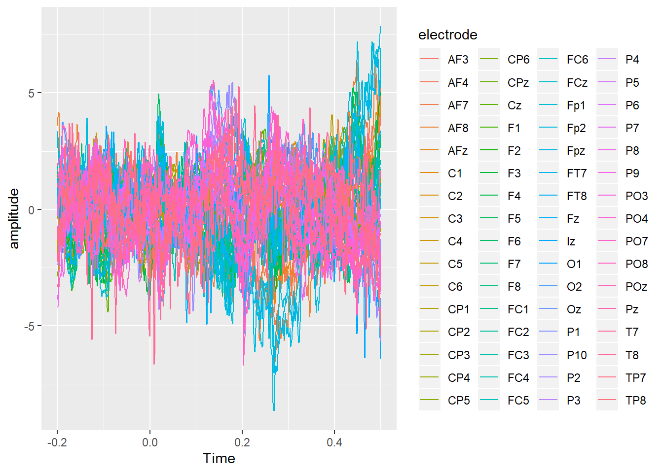

And here is a topography averaged from 150ms to 180ms after stimulus onset, produced using the topoplot() function from my nascent eegUtils package.

library(eegUtils)

## Make sure to check for the latest development version at https://github.com/craddm/eegUtils!

## 
## Attaching package: 'eegUtils'

## The following object is masked from 'package:stats':
## 
##     filter

filter(ERPs, Time >= .150 & Time <= .180) %>%
  topoplot()

## Attempting to add standard electrode locations...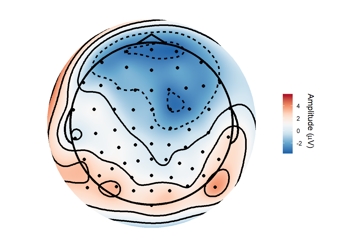

There are still, of course, more things we’d like to do. Normally we’d be doing some kind of artefact rejection - either rejecting trials with nasty artefacts manually or using some kind of algorithm such as FASTER or SCADS, or running Independent Component Analysis and using it to remove blinks and other artefact components.

At the moment, you’re totally on your own if trying to do this in R. There are ICA implementations in R but not really tailored to EEG data, and nothing like FASTER or SCADS is out there…yet!