EEG processing with Python, but in R: redux
Two years ago I wrote a post demonstrating Python pre-processing of EEG data using Python chunks in an RMarkdown document. This worked great. But something I mentioned then was that there was a package called reticulate that would allow more direct interfacing with Python in R. That package has been under a lot of development since then, as has RStudio. Plots produced in Python chunks can now be embedded in RMarkdown. The environment is now also shared between Python and R, whereas previously you couldn’t access something from a Python chunk in an R chunk and vice versa without going through the filesystem.
MNE-R is new package from the MNE-Python folks that’s intended to make things easier. For now it mostly ensures you import the MNE-Python library using reticulate. Thereafter, you’re using reticulate to interact with Python. It’s necessary to have a Python and MNE-Python installed separately - I recommend using Anaconda to manage this, and see here for more details on installing MNE-Python itself.
Once that’s done, we can begin!
Here I make sure reticulate is pointed at the correct conda enviroment using the use_condaenv() function, then import a couple of useful Python and R libraries. Note that I force matplotlib to use the “agg” backend. I’ve had no end of trouble with other backends. A downside of this is that currently you can’t really use the interactive elements of MNE-Python effectively, as they have a tendency to crash RStudio (at least on Windows).
library(reticulate)
use_condaenv(condaenv = "mne")
library(mne)
## Importing MNE version=0.18.dev0, path='C:\Users\Matt\ANACON~1\envs\mne\lib\site-packages\mne'mpl <- import("matplotlib")
mpl$use("agg") # On Windows at least, backends other than Agg tend to cause trouble...
plt <- import("matplotlib.pyplot")
library(eegUtils)
library(tidyverse)I’m going to use MNE to load in some raw BDF files and preprocess them.
example_files <-
  list.files("F:\\Users\\Matt\\Extero\\",
             pattern = "SSDT",
             full.names = TRUE)

eogChans <- list("EXG1", "EXG2", "EXG3", "EXG4")
miscChans <- list("EXG5", "EXG6", "EXG7", "EXG8")

proc_data <- function(x) {
  raw <- mne$io$read_raw_edf(x,
                             preload = TRUE,
                             eog = eogChans,
                             misc = miscChans)
  raw$info["bads"] <- list("EXG7", "EXG8")
  picks <- mne$pick_types(raw$info,
                          meg = FALSE,
                          eeg = TRUE,
                          eog = FALSE,
                          exclude = 'bads')
  raw <- raw$filter(1, 45)
  events <- mne$find_events(raw)
  events <- apply(events, 2, as.integer)
  raw$set_montage(mne$channels$read_montage('biosemi64'))
  raw$set_eeg_reference()
  event_id <- list("light" = 100L,
                   "no light" = 128L)
  tmin <- -.2
  tmax <- .5
  epoched_data <- mne$Epochs(raw,
                             events = events,
                             event_id = event_id,
                             tmin = tmin,
                             tmax = tmax,
                             preload = TRUE,
                             decim = 4L,
                             picks = as.integer(picks))
  epoched_data
}

all_raw <- lapply(example_files,
                  function(x) proc_data(x))

unclean_epochs <- mne$concatenate_epochs(all_raw) # note all_raw is an R list that is converted automatically!
Now we’ve collected all our data into a single Python object. Let’s take advantage of some of the other features available in Python and run AutoReject to automatically clean our imported and filtered EEG data.
autoreject <- import("autoreject")
picks <- as.integer(mne$pick_types(unclean_epochs$info,
                                   eeg = TRUE,
                                   eog = FALSE,
                                   exclude = 'bads'))
ar <- autoreject$AutoReject(thresh_method = 'random_search',
                            picks = picks,
                            random_state = 42L)
clean_epochs <- ar$fit_transform(unclean_epochs)
unclean_evoked <- unclean_epochs$apply_baseline(tuple(-.1, 0))$average()
clean_evoked <- clean_epochs$apply_baseline(tuple(-.1, 0))$average()
We can easily embed MNE’s own plots of this data using Python chunks:
r.unclean_evoked.plot_joint()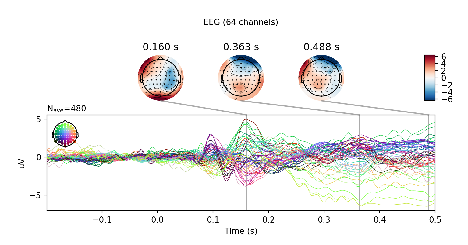
r.clean_evoked.plot_joint()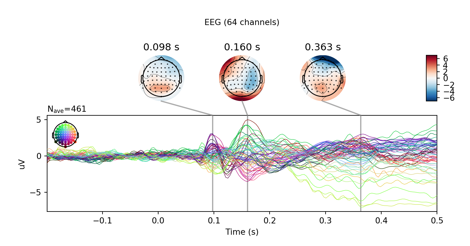
But of course, this is R-land!
A fun thing is that since the objects are fully accessible directly from R, we can use the MNE objects’ “to_data_frame()” methods to convert them to data frames, then pipe those data frames straight into tidyverse functions. Here I’ll take the clean epochs, convert them to long format, average them but keep the conditions separate, then plot them using ggplot2.
clean_epochs$to_data_frame(long_format = TRUE) %>%
  filter(ch_type == "eeg",
         time >= -100,
         time <= 400) %>%
  group_by(condition,
           time,
           channel) %>%
  summarise(amplitude = mean(observation)) %>%
  ggplot(aes(time,
             amplitude,
             colour = channel)) +
  stat_summary(geom = "line",
               fun.y = mean) +
  facet_wrap(~condition) +
  theme_minimal() +
  guides(color = FALSE) +
  labs(x = 'time [ms]',
       y = expression(paste("Amplitude (", mu, "V)"))) +
  theme(text = element_text(size = 20))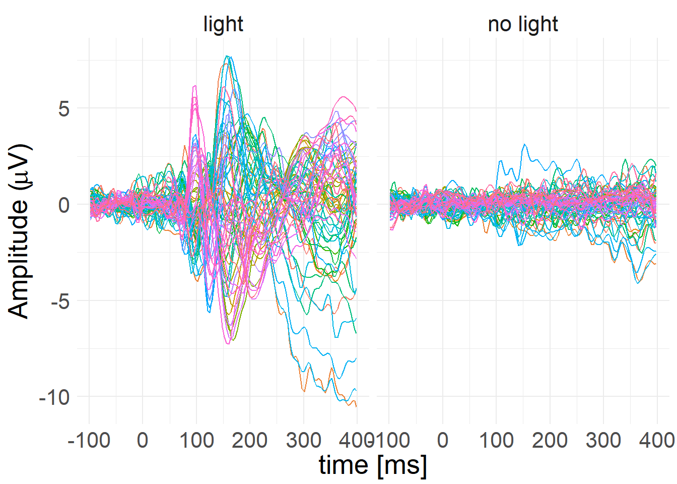
Since some functions from the eegUtils package support data frames, we can also easily use some of those functions on the resulting data. For example, here I use functions to add standard electrode locations to the data and then create a topographical plot using a custom geom, geom_topo. Note this version, using custom geoms, doesn’t have contours on yet, but we could also use the topoplot() function, which does.
clean_epochs$to_data_frame(long_format = TRUE,
                           picks = picks) %>%
  rename(electrode = channel,
         amplitude = observation) %>%
  electrode_locations() %>%
  filter(time >= 198, time <= 200) %>%
  ggplot(aes(x = x,
             y = y,
             fill = amplitude)) +
  geom_topo(interp_limit = "head",
            interpolate = TRUE) + # Interpolate smooths the raster plot
  scale_fill_distiller(palette = "RdBu") +
  theme_void() +
  guides(fill = guide_colorbar(title = expression(paste("Amplitude (",
                                                        mu, "V)")),
                                 title.position = "right",
                                 barwidth = rel(1),
                                 barheight = rel(6),
                                 title.theme = element_text(angle = 270))) +
coord_equal() 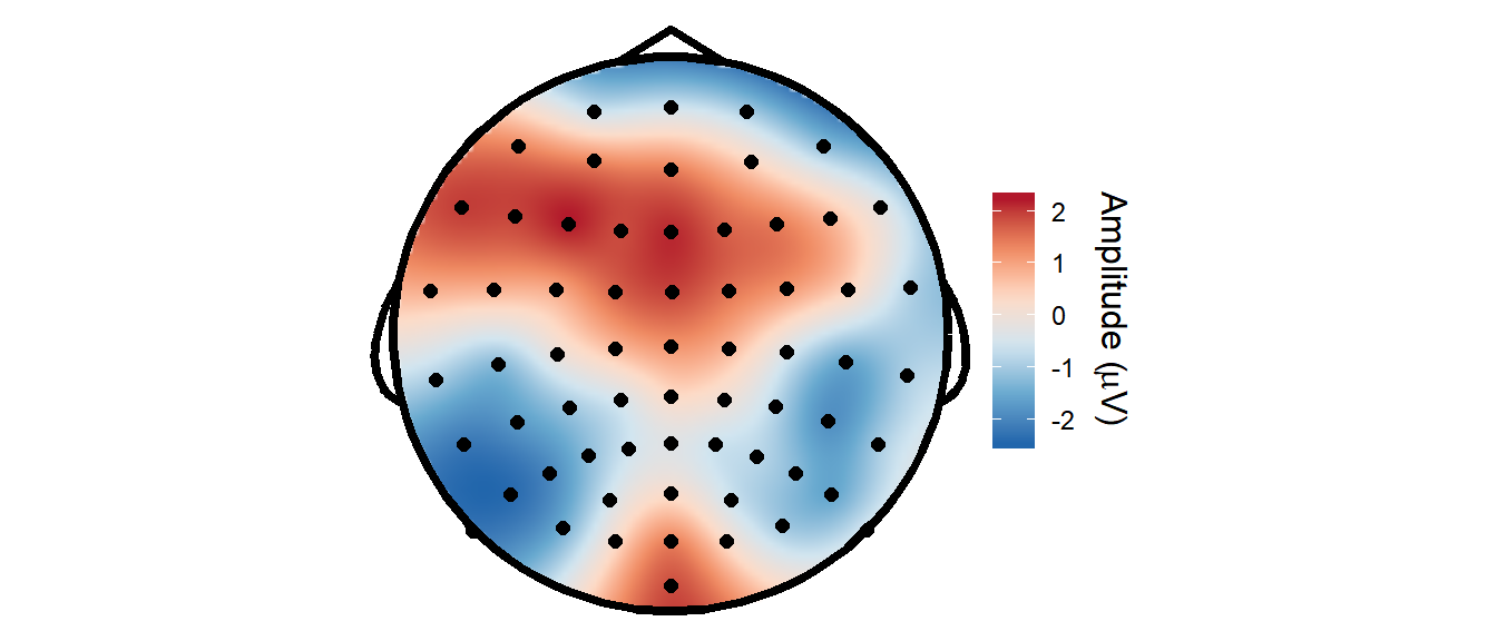
And here’s the same plot produced directly using MNE-Python.
r.clean_evoked.plot_topomap(times=.199)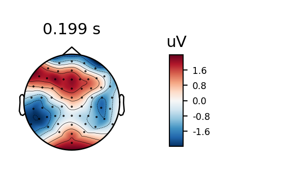
Interoperability between Python and R is now getting really easy, and it’s really exciting to be able to fluently switch between the two languages within a single document, passing structure to and from each language as and when necessary. And now that MNE-R is getting started, it’s going to get easier and easier!
Matt Craddock
I'm a research software engineer