What is intertrial coherence?

Calculating ITC

To be able to calculate ITC, we’re going to need the Fourier coefficients for every single trial.

demo_tfr <- compute_tfr(demo_epochs, 
                        foi = c(4, 30),
                        n_freq = 27,
                        n_cycles = 3,
                        keep_trials = TRUE,
                        output = "fourier")

## Output frequencies: 4 5 6 7 8 9 10 11 12 13 14 15 16 17 18 19 20 21 22 23 24 25 26 27 28 29 30

## Removing channel means per epoch...

Let’s have a look at raw power at all of the electrodes. Fourier coefficients can be converted to power by taking their absolute values and squaring them. plot_tfr() does that for us automatically.

plot_tfr(demo_tfr) +
  facet_wrap(~electrode)

## Data is complex Fourier coefficients, converting to power.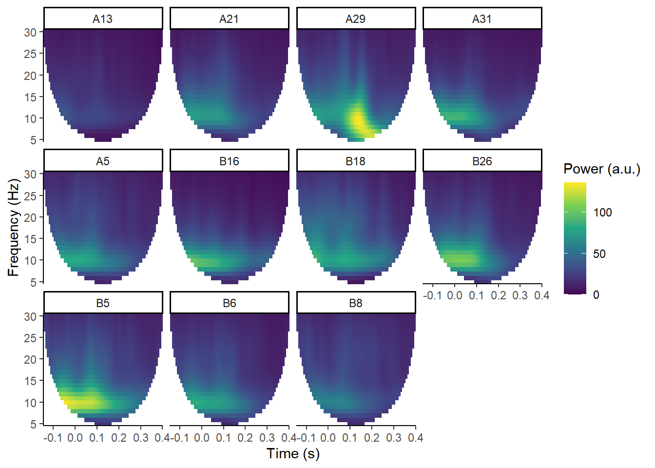

These plots show total power at the 11 electrodes in this data.

Ignore all the white at the edges; that’s just where the edges have been removed to avoid edge effects from the convolution process. This data is a bit short for demoing TFRs, but it’ll do for our purposes. You should be able to pick out that at A29 (roughly, Oz), there’s a post-stimulus power peak. That corresponds to the timing of a visual ERP.

Instead of taking the steps above, let’s convert our Fourier coefficients to phase angles. When we convert to phase angles, we set the magnitude to 1, placing phase on the unit circle. We can draw a polar plot, showing the position of each of the phase angles on that circle.

Let’s pick a single time point from the A29 electrode. I’ll pick out the Fourier coefficients from one timepoint, approximately 178 ms after stimulus onset, at 10 Hz.

demo_tfr$timings$time[49]

## [1] 0.1777344

all_fourier <- demo_tfr$signals[, 49, 4, 7]
phase_angle <- Arg(all_fourier)
circ.plot(phase_angle)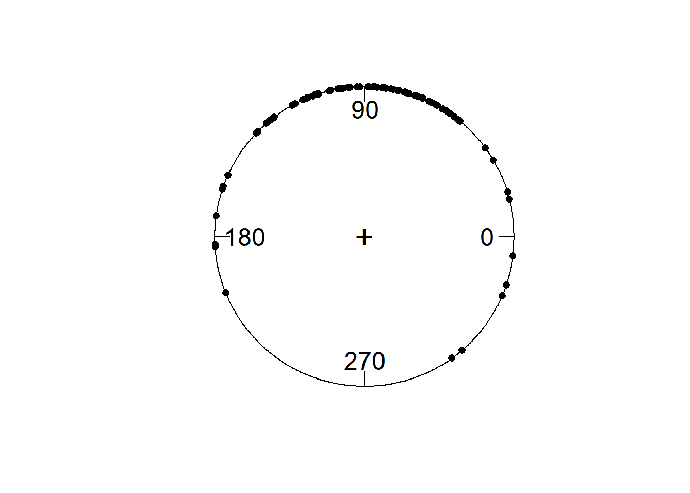

Each dot represents phase at a single time-point on a single trial.

ITC is a measure of how much those points cluster together. Something apparent from this plot is that there are many more phase angles around 90 degrees then there are around 270. If we wanted to know the average phase angle, we’d have to calculate the circular mean. Unlike amplitude, phase is a circular variable, just like time, or the degrees on a compass. Thus, 360 degrees and 0 degrees are the same; 359 degrees and 1 degree are 2 degrees apart, not 358 degrees.

circ.mean(phase_angle)

## [1] 1.56209

Note this is in radians rather than degrees.

But for ITC, the phase angles themselves are not so relevant. What matters is how dispersed they are around the circle.

Converting to ITC

Let’s convert the formula above to R code and calculate ITC at our single representative timepoint:

abs(sum(all_fourier / abs(all_fourier)) / length(all_fourier))

## [1] 0.7334559

We have an ITC of ~.73! That’s pretty high.

Now, with a few more lines of code, I’ll convert all the data to inter-trial coherence, and plot ITC at A29.

demo_ITC <- compute_ITC(demo_tfr)
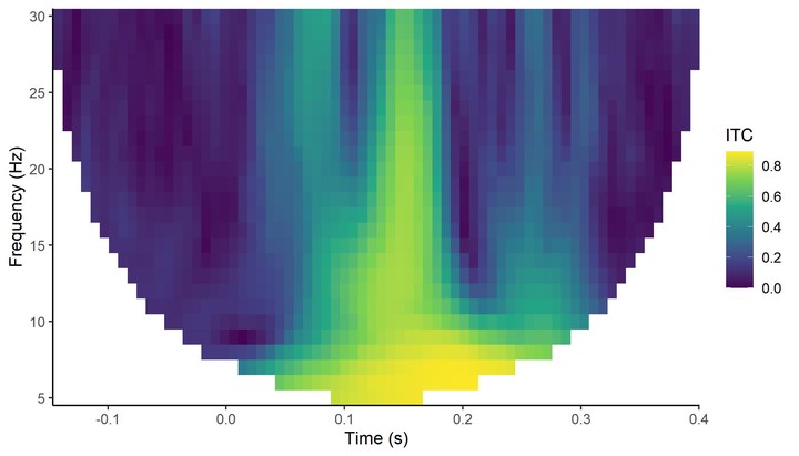
plot_tfr(demo_ITC, electrode = "A29") +
  labs(fill = "ITC")

From this we can see the phase of the oscillations recorded at A29 seems to align much more strongly across trials at around 150-180 ms, across most frequencies. This is approximately the time at which the ERPs to visual stimuli are peaking.

plot_timecourse(demo_epochs,
                "A29", 
                baseline = c(-.1, 0))

## Joining, by = c("epoch", "recording", "epoch_label", "participant_id")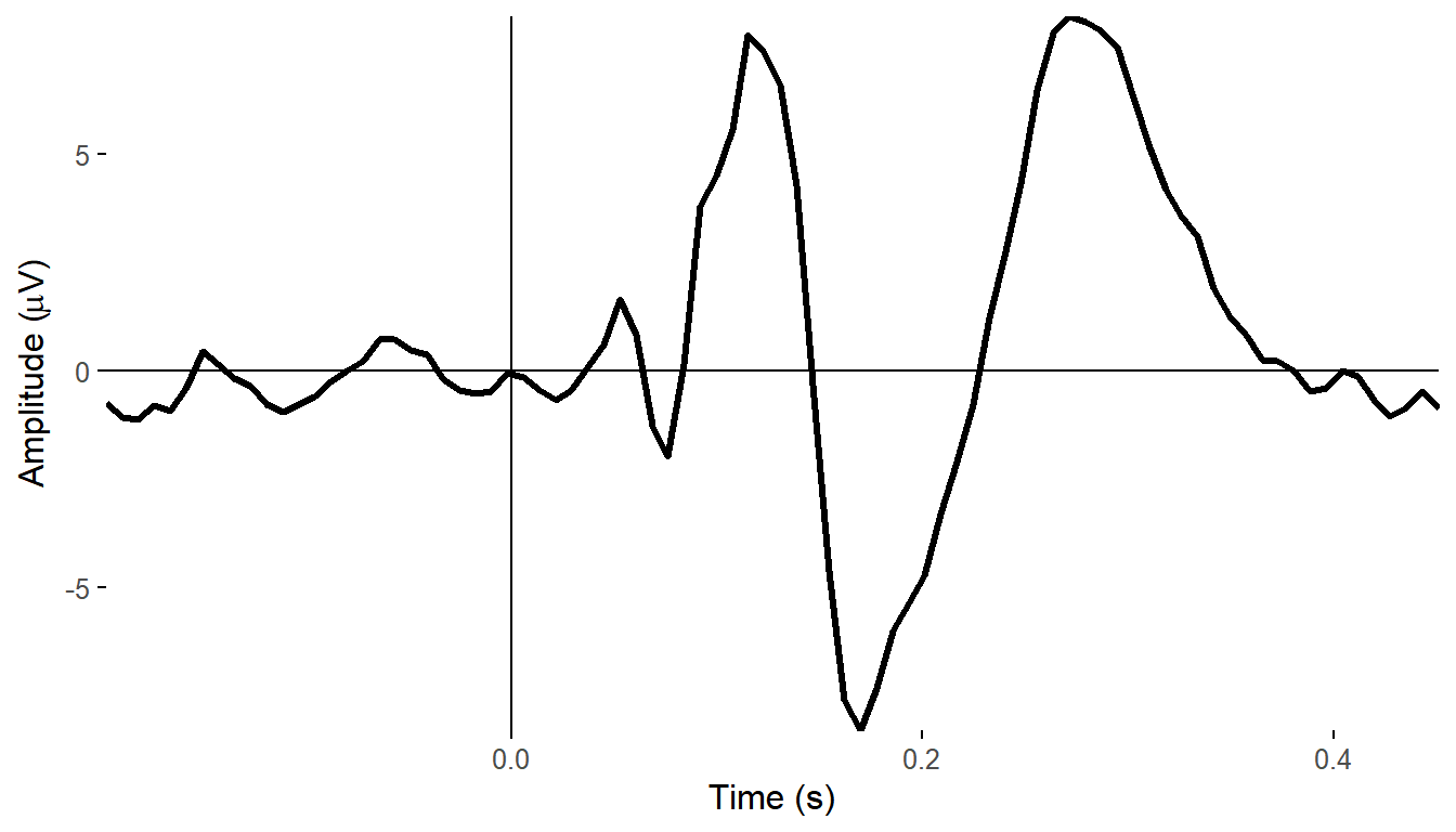

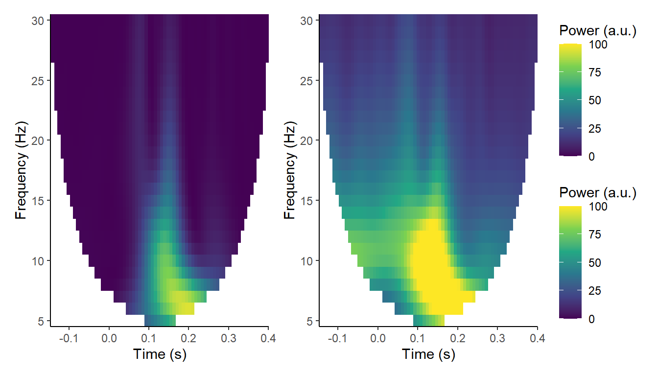
Thus, one interpretation of ITC is that it is capturing what we’d call evoked power - the power of the ERP - (left panel below) as opposed to induced or total power (right panel below). It is teasing out the phase-locked as opposed to non-phase-locked activity.

One thing to bear in mind is that ITC is a compound measure, a summary statistic that doesn’t in and of itself exist on a single-trial level. There have been several articles recently attempting to overcome this using a technique called jackknifing to relate it to single-trial behavioural measures such as reaction times. I’ll be looking at that in another post.