Loading EEGLAB .set files in R - part 2
In the last post, I showed how you can get the EEG data from EEGLAB .set files saved as Matlab v7.3 files, but that there are some limitations on what else you can get from them beyond the data itself. Specifically, you can’t extract channel locations, and there are no labels to tell you which channels the data is from. This is due a limitation of the available tools for reading HDF5 files, which is the actual format of Matlab v7.3 files.
If you save the file in Matlab v6.5 format, however, you don’t have the same problems.
EEGLAB .set files in v6.5 format
This time I saved the file with these two options ticked.
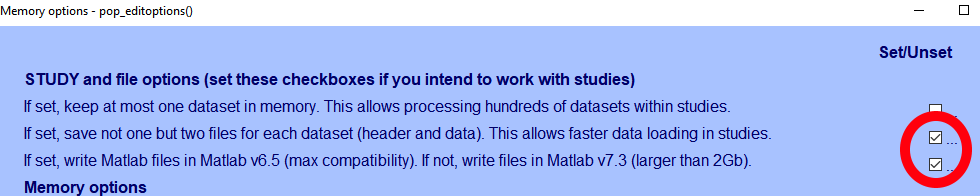
This splits the file in two: a .set file contains the EEG structure but not the data, while a .fdt file contains the EEG data but not the rest of the structure.
I generally use this method of saving as it results in smaller files.
Anyway, for files in older Matlab formats, you can use the R.matlab package.
library(R.matlab)## R.matlab v3.6.2 (2018-09-26) successfully loaded. See ?R.matlab for help.##
## Attaching package: 'R.matlab'## The following objects are masked from 'package:base':
##
## getOption, isOpenfile_name <- "HSFObj_v6.set"
EEG <- readMat(file_name)All the meat is in the first element of the resulting list, which in this case is an element called EEG, the name of the structure that was saved by EEGLAB.
EEG$EEG## , , 1
##
## [,1]
## setname "S18MatchHSFObj.set"
## filename "HSFObj_v6.set"
## filepath "C:\\Users\\Matt\\Documents\\GitHub\\hugo-blog\\content\\post"
## subject Character,0
## group Character,0
## condition Character,0
## session Numeric,0
## comments Character,7
## nbchan 68
## trials 54
## pnts 717
## srate 512
## xmin -0.4003906
## xmax 0.9980469
## times Numeric,717
## data "HSFObj_v6.fdt"
## icaact Numeric,0
## icawinv Numeric,0
## icasphere Numeric,0
## icaweights Numeric,0
## icachansind Numeric,0
## chanlocs List,816
## urchanlocs Numeric,0
## chaninfo List,7
## ref "averef"
## event List,648
## urevent List,5782
## eventdescription List,4
## epoch List,216
## epochdescription List,0
## reject List,38
## stats List,13
## specdata Numeric,0
## specicaact Numeric,0
## splinefile Character,0
## icasplinefile Character,0
## dipfit Numeric,0
## history "\nEEG = eeg_checkset( EEG );\nEEG = eeg_checkset( EEG );\nEEG = eeg_checkset( EEG );\nEEG = eeg_checkse" [truncated]
## saved "yes"
## etc List,1
## datfile "HSFObj_v6.fdt"Unlike in the last post, all of this information is accessible. To get at individual parts, you can address them directly. If I’d have saved the .set file as one file, then the data itself would be contained in the data field, which is the 16th element of the list. Here, instead, it has the name of the .fdt datafile.
EEG$EEG[[16]]## [,1]
## [1,] "HSFObj_v6.fdt"That’s a simple binary file, not a .mat file, so to load the .fdt in we’ll need to use some of the low-level file reading commands.
fdt_name <- unlist(EEG$EEG[[16]])
fdt_name
## [,1]
## [1,] "HSFObj_v6.fdt"fdt_file <- file(fdt_name, "rb")To know what shape matrix the .fdt file contains, we need to now the number of channels, number of trials, and number of timepoints per trial. Those are all available from the .set file we already loaded. Rather than having to count out which element to address each time, what I like to do is extract the dimension names from the list use which() to find the appropriate number.
var_names <- dimnames(EEG$EEG)[[1]]
var_names
## [1] "setname" "filename" "filepath" "subject"
## [5] "group" "condition" "session" "comments"
## [9] "nbchan" "trials" "pnts" "srate"
## [13] "xmin" "xmax" "times" "data"
## [17] "icaact" "icawinv" "icasphere" "icaweights"
## [21] "icachansind" "chanlocs" "urchanlocs" "chaninfo"
## [25] "ref" "event" "urevent" "eventdescription"
## [29] "epoch" "epochdescription" "reject" "stats"
## [33] "specdata" "specicaact" "splinefile" "icasplinefile"
## [37] "dipfit" "history" "saved" "etc"
## [41] "datfile"n_chans <- EEG$EEG[[which(var_names == "nbchan")]]
n_trials <- EEG$EEG[[which(var_names == "trials")]]
times <- EEG$EEG[[which(var_names == "times")]]Loading the data is straightforward using the readBin() command. EEGLAB saves the data as 32-bit floating point numbers. That type of number is a “double” of size 4 (bytes) in readBin terms. The number of records is the number of channels times the number of trials the the number of timepoints.
signals <- readBin(fdt_file,
                   "double",
                   n = n_chans * n_trials * length(times),
                   size = 4,
                   endian = "little")
close(fdt_file)
We then reshape the signals to a matrix with the correct dimensions. Note that if the data was contained in the .set file, they will already be in a matrix with the correct dimensions. I’ll only print the first 5 columns to keep the output short.
dim(signals) <- c(n_chans, length(times) * max(n_trials, 1))
times <- rep(times, max(n_trials, 1))
signals <- data.frame(cbind(t(signals), times))
head(signals[, 1:5])
## V1 V2 V3 V4 V5
## 1 6.106716 8.514810 7.018276 0.8339983 6.546292
## 2 5.268877 7.200565 6.019012 -0.1963540 6.032383
## 3 3.866934 5.163206 3.676486 -0.8304622 5.306540
## 4 2.242807 4.115035 1.201425 -1.2985356 4.252594
## 5 1.922712 5.439950 1.097038 -1.4731051 3.497955
## 6 3.008378 8.099439 3.036014 -0.9918253 3.753252So, now we have data frame in wide format - a column for each electrode, and a final column givin the time of each sample within each epoch. But the electrode columns just have generic names (V1:V68). To figure out which one is which, we need information from chanlocs.
chanlocs is the 22nd element of the EEG list.
var_names <- dimnames(EEG$EEG)[[1]]
var_names
## [1] "setname" "filename" "filepath" "subject"
## [5] "group" "condition" "session" "comments"
## [9] "nbchan" "trials" "pnts" "srate"
## [13] "xmin" "xmax" "times" "data"
## [17] "icaact" "icawinv" "icasphere" "icaweights"
## [21] "icachansind" "chanlocs" "urchanlocs" "chaninfo"
## [25] "ref" "event" "urevent" "eventdescription"
## [29] "epoch" "epochdescription" "reject" "stats"
## [33] "specdata" "specicaact" "splinefile" "icasplinefile"
## [37] "dipfit" "history" "saved" "etc"
## [41] "datfile"chanlocs <- EEG$EEG[[which(var_names == "chanlocs")]]
dim(chanlocs)## [1] 12 1 68Chanlocs comes out as a 3D list with 12 * number_of_chans elements, with each list element itself a list. These 12 elements include things such as the electrode label, and x/y co-ordinates. The 3rd dimension is channels/electrodes, so we can get the information for a single channel by addressing that 3rd dimension. That gives use a list of 12 elements, which we can combine into a single row using rbind().
rbind(chanlocs[, , 1])## labels theta radius X Y Z sph.theta sph.phi
## [1,] "Fp1" -18 0.5111111 80.69551 26.21956 -2.962967 18 -2
## sph.radius type ref urchan
## [1,] 84.9 "1" "average" 1What’d be nice is to end up with a data frame or tibble with a row like the above for each electrode, which we can accomplish with some more rbind magic.
chanlocs <- as.data.frame(t(rbind(chanlocs[, , ])))
head(chanlocs)
## labels theta radius X Y Z sph.theta sph.phi
## 1 Fp1 -18 0.5111111 80.69551 26.21956 -2.962967 18 -2
## 2 AF7 -36 0.5111111 68.6437 49.87257 -2.962967 36 -2
## 3 AF3 -25 0.4111111 73.96479 34.49035 23.40161 25 16
## 4 F1 -22 0.2777778 60.30142 24.36335 54.57267 22 40
## 5 F3 -39 0.3333333 57.14009 46.27113 42.45 39 30
## 6 F5 -49 0.4166667 53.8015 61.89155 21.97374 49 15
## sph.radius type ref urchan
## 1 84.9 1 average 1
## 2 84.9 2 average 2
## 3 84.9 3 average 3
## 4 84.9 4 average 4
## 5 84.9 5 average 5
## 6 84.9 6 average 6Irritatingly, that’s ended up as a data frame full of lists, which isn’t immediately obvious until you try to use any of it and find it painfully awkward to do so. It’s more obvious when a tibble is used instead of a data.frame.
library(tibble)
head(as_tibble(chanlocs))
## # A tibble: 6 x 12
## labels theta radius X Y Z sph.theta sph.phi sph.radius type ref
## <list> <lis> <list> <lis> <lis> <lis> <list> <list> <list> <lis> <lis>
## 1 <chr[… <dbl… <dbl[… <dbl… <dbl… <dbl… <dbl[,1]… <dbl[,… <dbl[,1] … <chr… <chr…
## 2 <chr[… <dbl… <dbl[… <dbl… <dbl… <dbl… <dbl[,1]… <dbl[,… <dbl[,1] … <chr… <chr…
## 3 <chr[… <dbl… <dbl[… <dbl… <dbl… <dbl… <dbl[,1]… <dbl[,… <dbl[,1] … <chr… <chr…
## 4 <chr[… <dbl… <dbl[… <dbl… <dbl… <dbl… <dbl[,1]… <dbl[,… <dbl[,1] … <chr… <chr…
## 5 <chr[… <dbl… <dbl[… <dbl… <dbl… <dbl… <dbl[,1]… <dbl[,… <dbl[,1] … <chr… <chr…
## 6 <chr[… <dbl… <dbl[… <dbl… <dbl… <dbl… <dbl[,1]… <dbl[,… <dbl[,1] … <chr… <chr…
## # … with 1 more variable: urchan <list>So finally I use lapply to iterate through the columns, unlisting them, and coercing them back into a data.frame.
chanlocs <- data.frame(lapply(chanlocs, unlist), stringsAsFactors = FALSE)
head(chanlocs)
## labels theta radius X Y Z sph.theta sph.phi
## 1 Fp1 -18 0.5111111 80.69551 26.21956 -2.962967 18 -2
## 2 AF7 -36 0.5111111 68.64370 49.87257 -2.962967 36 -2
## 3 AF3 -25 0.4111111 73.96479 34.49035 23.401612 25 16
## 4 F1 -22 0.2777778 60.30142 24.36335 54.572668 22 40
## 5 F3 -39 0.3333333 57.14009 46.27113 42.450000 39 30
## 6 F5 -49 0.4166667 53.80150 61.89155 21.973737 49 15
## sph.radius type ref urchan
## 1 84.9 1 average 1
## 2 84.9 2 average 2
## 3 84.9 3 average 3
## 4 84.9 4 average 4
## 5 84.9 5 average 5
## 6 84.9 6 average 6This works nicely here, but will fail if there are are any empty or NULL values in the lists. To guard against that, as a clunky way of doing it I first run through the whole list using lapply (from base R) and is_empty from the purrr package. lapply returns a flat list, so I have to tweak it a little to get it back in the a format where it’s easy to turn it into a data frame.
library(purrr)
chan_info <- EEG$EEG[[which(var_names == "chanlocs")]]
col_names <- dimnames(chan_info)[1]
size_chans <- dim(chan_info)
chan_info <- lapply(chan_info, function(x) ifelse(is_empty(x), NA,x ))
dim(chan_info) <- size_chans
dimnames(chan_info) <- col_names
chan_info <- tibble::as_tibble(t(as.data.frame(chan_info)))
chan_info <- tibble::as_tibble(data.frame(lapply(chan_info, unlist), stringsAsFactors = FALSE))
head(chan_info)
## # A tibble: 6 x 12
## labels theta radius X Y Z sph.theta sph.phi sph.radius type ref
## <chr> <dbl> <dbl> <dbl> <dbl> <dbl> <dbl> <dbl> <dbl> <chr> <chr>
## 1 Fp1 -18 0.511 80.7 26.2 -2.96 18 -2 84.9 1 aver…
## 2 AF7 -36 0.511 68.6 49.9 -2.96 36 -2 84.9 2 aver…
## 3 AF3 -25 0.411 74.0 34.5 23.4 25 16 84.9 3 aver…
## 4 F1 -22 0.278 60.3 24.4 54.6 22 40 84.9 4 aver…
## 5 F3 -39 0.333 57.1 46.3 42.4 39 30 84.9 5 aver…
## 6 F5 -49 0.417 53.8 61.9 22.0 49 15 84.9 6 aver…
## # … with 1 more variable: urchan <dbl>There’s bound to be a more elegant way, but this at least works…
Now we have a nice clean data frame containing all the info from the EEGLAB chanlocs structure.
Finally, we’ll extract the channel names and rename the columns in our signals data frame.
names(signals) <- c(chanlocs$labels, "times")
head(signals[, 1:5])
## Fp1 AF7 AF3 F1 F3
## 1 6.106716 8.514810 7.018276 0.8339983 6.546292
## 2 5.268877 7.200565 6.019012 -0.1963540 6.032383
## 3 3.866934 5.163206 3.676486 -0.8304622 5.306540
## 4 2.242807 4.115035 1.201425 -1.2985356 4.252594
## 5 1.922712 5.439950 1.097038 -1.4731051 3.497955
## 6 3.008378 8.099439 3.036014 -0.9918253 3.753252As a final trick, we’ll use dplyr to add epoch numbers.
library(dplyr)
signals <- signals %>%
  group_by(times) %>%
  mutate(epoch = 1:n()) %>%
  ungroup

head(signals[, 65:70])
## # A tibble: 6 x 6
## EXG1 EXG2 EXG3 EXG4 times epoch
## <dbl> <dbl> <dbl> <dbl> <dbl> <int>
## 1 -6.64 5.15 1.33 10.7 -400. 1
## 2 -7.36 7.32 0.295 9.71 -398. 1
## 3 -1.95 8.88 -1.26 10.0 -396. 1
## 4 2.66 6.06 -2.57 9.43 -395. 1
## 5 3.36 3.30 -2.56 8.43 -393. 1
## 6 1.56 5.49 -0.482 8.96 -391. 1Now we have a data frame in wide format, ready to be tidified if required, and suitable for further analysis as you wish.
And after all that, I’ve implemented the above as the command load_set() in my eegUtils package. By default it’ll return an eeg_data object rather than a data frame, but you can convert eeg_data objects to data frames using as.data.frame().
Matt Craddock
I'm a research software engineer