Jackknife intertrial coherence and phase

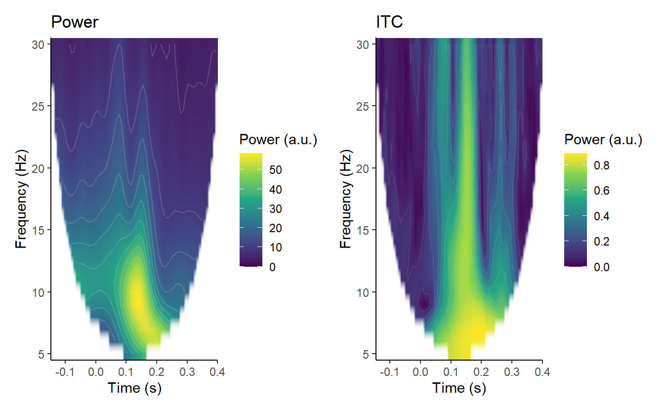
Single-trial, jackknife-ITC

Jackknifing is a method of estimating the bias and standard error of a parameter estimate (e.g. the mean of a set of observations) by recomputing the estimate from subsamples of the full sample.

For example, we take a full sample of data and calculate its mean. We then take all but one observation and calculate the mean again. We repeat this over and over, systematically leaving out one observation each time, until we have left out each observation once. Each of these repeats is called a leave-one-out jackknife replication. If the size of our sample is \(N\), there are \(N\) possible replications, and each replication is calculated from a sample of size \(N-1\).

The first step is to calculate jackknife replications. Basically, to figure out a partial estimate of ITC for each trial, we calculate what the ITC would be without that trial. Here I create a function to calculate ITC and then create jackknife replications, systematically leaving out each trial.

calculate_ITC <- function(x) {
  x <- abs(sum(x / abs(x))) / length(x)
}

all_fourier <- demo_tfr$signals[, 49, 4, 7] # 10 Hz, A29
ITC <- calculate_ITC(all_fourier)
ITC 

## [1] 0.7334559

jackknifed_ITC <- numeric(80)
for (i in seq(1, 80)) {
  jackknifed_ITC[i] <- calculate_ITC(all_fourier[-i])
}

There are 80 trials in this dataset, so this gives us 80 replications. The mean of those 80 replications is our jackknife estimate of ITC.

mean(jackknifed_ITC)

## [1] 0.7334869

hist(jackknifed_ITC)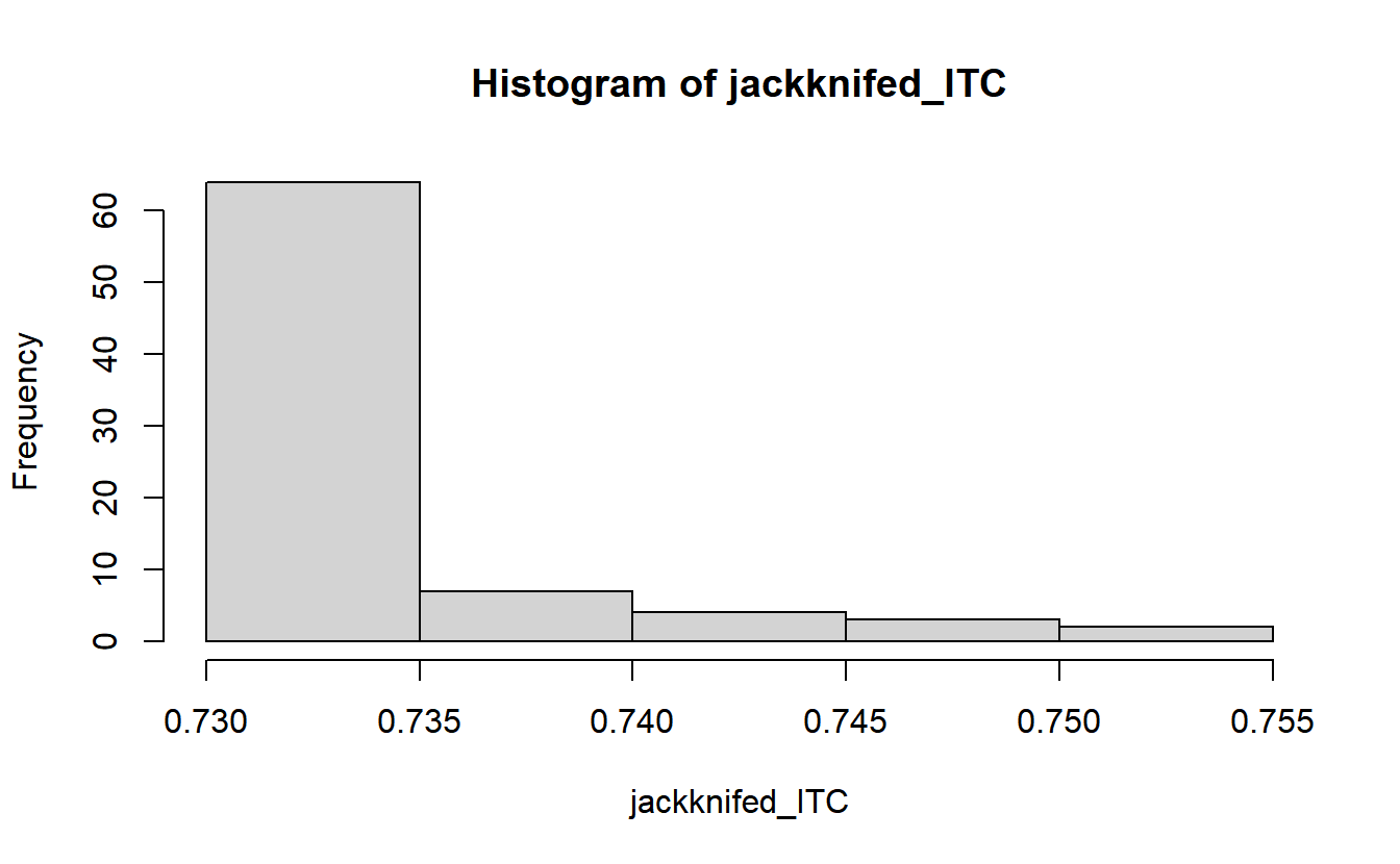

You need to use a little caution interpreting these values. Remember that these are the values that ITC would have had without one specific trial. Our all-trials ITC was .73, so when removing a single trial doesn’t really change ITC from that, it tells us that trial was quite similar to the rest. But when removing a trial really changes the ITC, that specific trial was quite different from the rest.

These can also be converted to jackknife pseudovalues.

pseudovals <- 80*ITC - (79*jackknifed_ITC)
hist(pseudovals)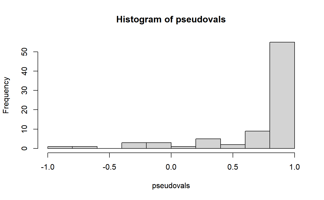

An article by Richter, Thompson, Bosman, and Fries (2015) examined how, using this approach, one could calculate the correlation between between statistics that don’t have single-trial values (such as coherence) and statistics that do (such as reaction times) by calculating the correlation between their jackknife replications.[^1]

So what does single-trial ITC actually mean?

The thing is, a question I had when I saw jackknifed ITC was - what does that actually mean? There are some jackknife-able variables that I think make theoretic sense. For example, sometimes a jacknife is used to calculate single trial sensitivity (d’). One can readily imagine that the underlying property, perceptual sensitivity, can exist on a single trial.

But ITC, by definition, has to be a property of multiple trials - it’s a measure of coherence across trials. How can we thus

Let’s take a step back. What exactly is ITC?

ITC is a measure of phase consistency/concentration. Let’s convert our Fourier coefficients to phase angles, using a polar plot that shows the position of each of the phase angles on the unit circle, and let’s calculate the mean phase.

phase_angle <- Arg(all_fourier)
circ.plot(phase_angle)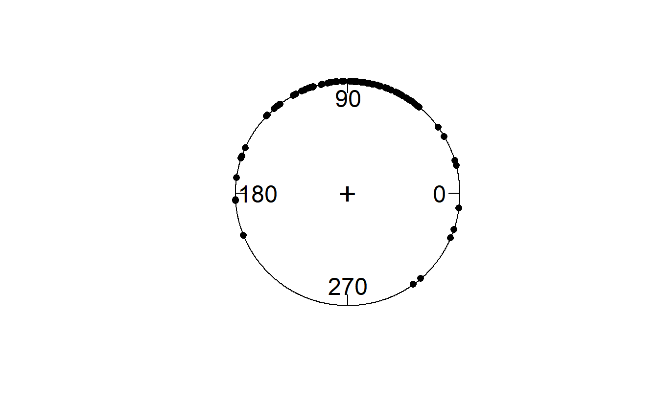

circ.mean(phase_angle)

## [1] 1.56209

This gives us a notion of the mean direction of phase (in this case, expressed in radians, rather than degrees).

But what about the variance around that mean? This is expressed by the circular variance, and its complement, the mean resultant length. The more concentrated the phase, the greater the mean resultant length. If all phases are the same, the mean resultant length is 1. If all phases are maximally spread around the unit circle, then it would be 0.

Let’s calculate that now:

circ.disp(phase_angle)

##    n        r      rbar       var
## 1 80 58.67647 0.7334559 0.2665441

The quantity rbar (\(\bar{r}\)) is the mean resultant length. Compare that to our ITC: it’s the same thing. And the circular variance - var - is \(1 - \bar{r}\).

So the mean resultant length/ITC is a measure of dispersion around the circular mean of the phase angles. And while ITC is not defined on a single-trial basis, phase is.

Phase and jackknifed ITC

Suppose, then, that we were to relate single-trial phase to jackknifed pseudovalues or jackknife replicates; what pattern would we see?

qplot(phase_angle,
      jackknifed_ITC) +
  geom_hline(yintercept = ITC) +
  geom_vline(xintercept = circ.mean(phase_angle))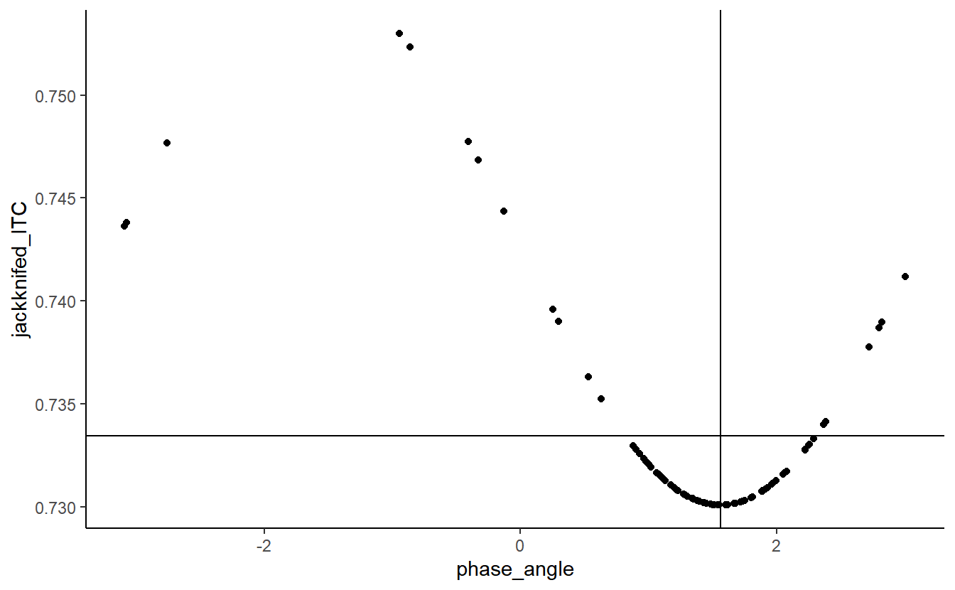

qplot(phase_angle,
      pseudovals) +
  geom_hline(yintercept = ITC) +
  geom_vline(xintercept = circ.mean(phase_angle))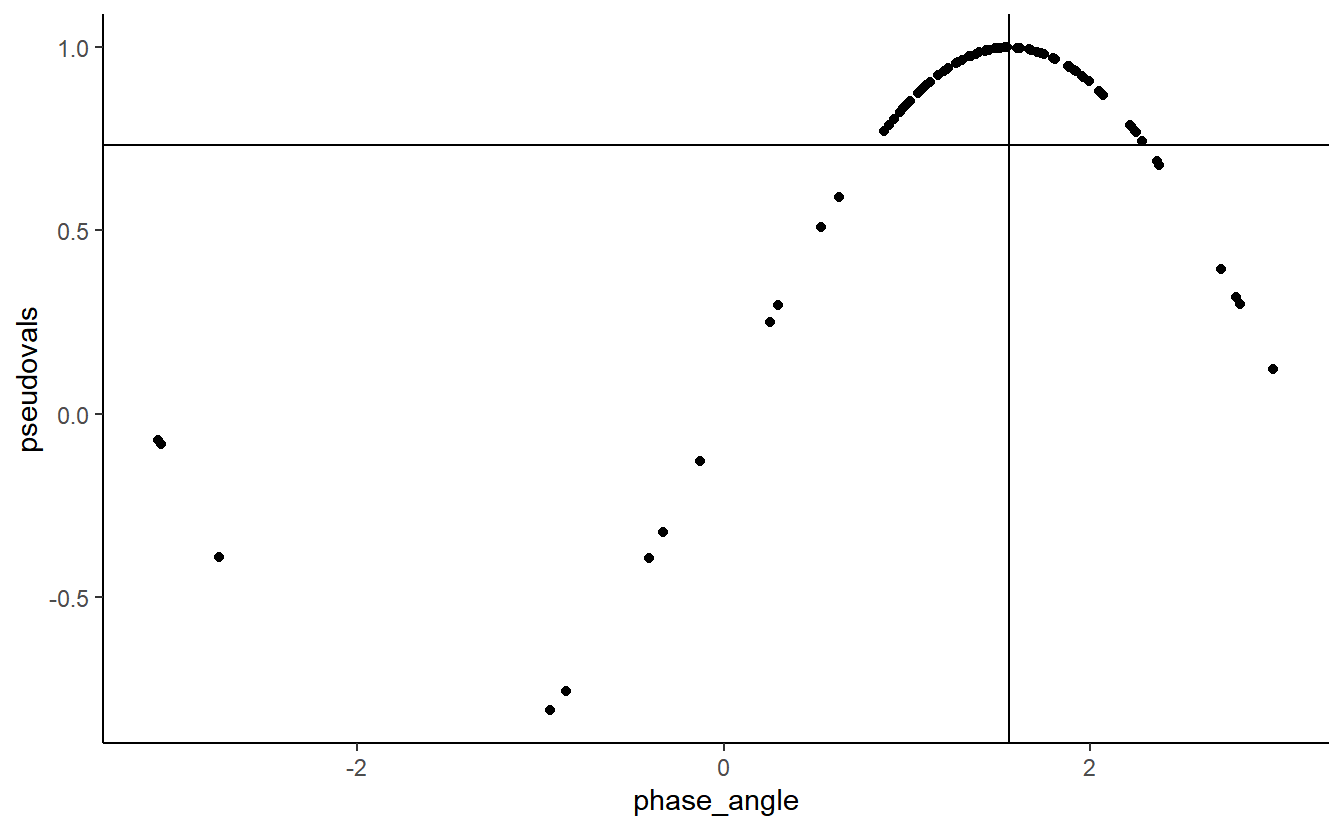

The relationship between the two is clearly sinusoidal.

We can enter a circular predictor into a linear model using its sine and cosine:

summary(lm(jackknifed_ITC ~ sin(phase_angle) + cos(phase_angle)))

## 
## Call:
## lm(formula = jackknifed_ITC ~ sin(phase_angle) + cos(phase_angle))
## 
## Residuals:
##        Min         1Q     Median         3Q        Max 
## -8.536e-05 -1.174e-05 -4.970e-06  1.070e-05  4.869e-05 
## 
## Coefficients:
##                    Estimate Std. Error   t value Pr(>|t|)    
## (Intercept)       7.428e-01  4.726e-06 157172.04   <2e-16 ***
## sin(phase_angle) -1.272e-02  5.593e-06  -2274.32   <2e-16 ***
## cos(phase_angle) -1.194e-04  4.400e-06    -27.15   <2e-16 ***
## ---
## Signif. codes:  0 '***' 0.001 '**' 0.01 '*' 0.05 '.' 0.1 ' ' 1
## 
## Residual standard error: 2.096e-05 on 77 degrees of freedom
## Multiple R-squared:      1,  Adjusted R-squared:      1 
## F-statistic: 2.598e+06 on 2 and 77 DF,  p-value: < 2.2e-16

Note that the \(r^2\) is 1. Thus, jackknifed ITC, a quantity that is calculated because ITC is undefined on the single-trial level, is actually a transformation of phase, which is defined on the single-trial level. Perhaps the simplest way to show this is by centring our distribution of phase angles on their mean:

cent_phase_angle <- phase_angle - circ.mean(phase_angle)
wrapp_phase <- ifelse(abs(cent_phase_angle) >  pi,
                      cent_phase_angle + 2*pi,
                      cent_phase_angle)
qplot(wrapp_phase,
      pseudovals) +
  geom_hline(yintercept = ITC) +
  theme_classic()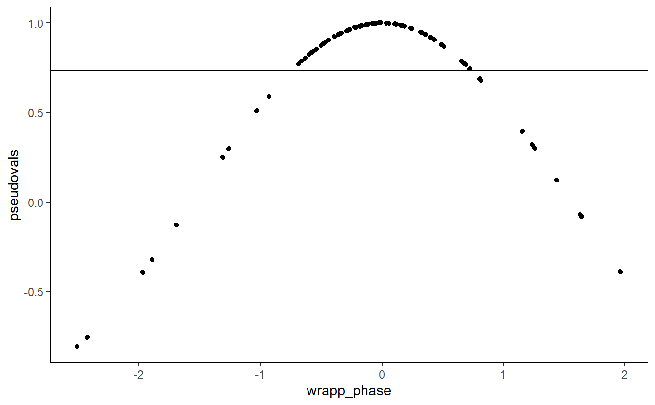

Jackknifed ITC is a transformation of a trial’s absolute difference from mean phase. The further away a trial’s phase is from the mean phase, the greater the jackknife ITC.

[^1] Note that a caveat is that one should use jackknife estimates of both parameters, even the ones that do exist on the single trial level. i.e. you calculate the jackknife estimate of both ITC and mean RT when a given trial is left out.